Several months ago, I worked with Professor David Corso and his team at the University of Michigan on an MDP Project to subdivide newspaper articles from full newspaper sheets. Our project revolved around analyzing a newspaper sheet, identifying each of the articles within that sheet, and saving each article to a unique file. The purpose of the exercise was to allow downstream applications to run OCR on the subdivided images to improve OCR quality and ultimately improve search relevancy.

In the months that followed, I crossed paths with a number of additional image segmentation tasks in Yale’s Digital Humanities Lab, all of which seemed to suggest that image segmentation is an area of increasing importance in digital research. Given the paucity of material on image segmentation, I thought it would be worthwhile to write up a quick case study that shows how one can perform some simple image segmentation.

Case Study: Segmenting playbills

The case study discussed below grows out work I pursued when the British Library asked if Yale’s Digital Humanities Lab could help process a large image collection in their possession. Their data consisted of scrapbooks wherein each page/image contained several advertisements for eighteenth-century plays. Here’s a sample image:

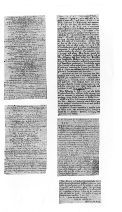
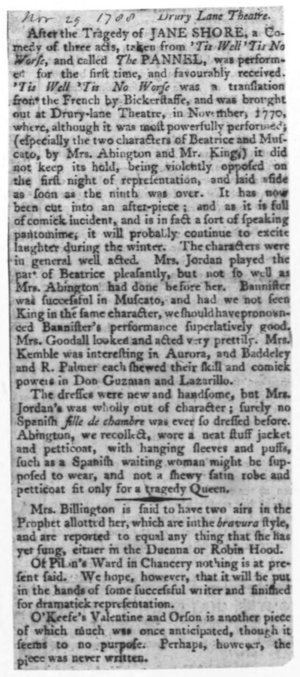
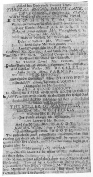
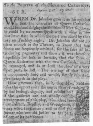
Given an image such as the above, they wanted to save each of the clippings from that page to its own file:

This is a fairly tidy example of an image segmentation task, and one that our lab achieved quickly with Python’s scikit-image package. The write-up below documents the approaches we leveraged for this task.

Converting an image file to a pixel matrix

To get started, one must first install skimage. To do so, just open a terminal and type pip install scikit-image. From there, one can read a jpg or jp2 into RAM with a script such as the following:

from skimage import io
from scipy import ndimage
import sys

image_file = sys.argv[1]
file_extension = image_file.split(".")[-1]

if file_extension in ["jpg", "jpeg"]:
  im = ndimage.imread(image_file)

elif file_extension in ["jp2"]:
  im = io.imread(image_file, plugin='freeimage')

else:
  print("your input file isn't jpg or jp2")
  sys.exit()

To invoke this script, save the above to a file (e.g. image_segmentation.py) and run: python image_segmentation.py PATH_TO/AN_IMAGE.jpg, where the sole argument provided to the script is the path to an image file on your machine.

If you do so, you’ll instantiate an im object. If you print that object, you’ll see it’s a matrix. The shape of this matrix depends on the input image type, as discussed in the relevant scipy and skimage docs. In the case of the grayscale images above, the im object is a 2d matrix, or array of arrays. Each subarray represents one row of pixels in the image, and each integer in a given subarray represent the luminescence of a pixel in the given row in 8bit scale (0 = black, 255 = white):

>>> print(im)
[[255 255 255 ..., 255 255 255]
 [255 255 255 ..., 255 255 255]
 [255 255 255 ..., 255 255 255]
 ...,
 [254 254 254 ..., 255 255 255]
 [254 254 254 ..., 255 255 255]
 [254 254 254 ..., 255 255 255]]

One can run a wide range of numerical operations on this image pixel matrix in order to achieve different tasks. Below we’ll look at two approaches one can use to save each subimage in a composite image to its own file.

Image segmentation with pixel dilations

One approach that’s often useful in image processing is “pixel dilation.” This term refers to the process of measuring the total amount of luminescence for each row and each column of an image. Measuring these values can provide helpful inputs with which one can automatically crop or even segment image elements.

Given a matrix representation of the composite image discussed above, for example, one can easily find the aggregate luminesence of each column of pixels. The plot below on the right visualizes the aggregate luminesence of each column of pixels for the image on the left below:

Examining this chart, we can tell there are two dark bands of pixels within the image on the left: one that stretches from roughly pixels 100-800 in the image, and another that stretches from roughly 1200-1900. Given just this representation of the image’s contents, one would have enough information to partition the image into two regions. From there, one could repeat the procedure, this time dilating pixels along the y axis and again splitting the image based on the resulting blocks within the pixel histogram.

To generate pixel histograms such as the one above for the x and y axes of an image matrix named im, one can run:

# plot the amount of white ink across the columns & rows
row_vals = list([sum(r) for r in im  ])
col_vals = list([sum(c) for c in im.T])

# plot the column (x-axis) pixel dilations
plt.plot(col_vals)
plt.show()

# plot the row (y-axis) pixel dilations
plt.plot(row_vals)
plt.show()

Image segmentation with pixel clustering

While pixel dilations can offer significant clues for image processing, many image segmentation tasks involve identifying non-rectilinear patterns, and therefore require more flexible solutions. Below we’ll examine one approach to automatically segmenting an image into discrete regions of interest.

Binarizing grayscale pixels

The sample image discussed above is an 8bit grayscale image. Each pixel is represented as an integer value between 0 and 255, where 0 = perfect black and 255 = perfect white. One way to simplify image processing for this kind of color scale is to “binarize” the image, or transform the image such that each pixel is either black or white.

To binarize a grayscale image, we simply need to identify a threshold value between 0 and 255. Once the threshold is established, we can identify each pixel with a boolean (True/False) value that indicates whether the given pixel is black/white. As it happens, the threshold_otsu() function in skimage provides a helper for determining an ideal threshold value for binarizing a grayscale image, and the clear_border() method provides a helper for applying a binarized image mask to an image:

from skimage import filters, segmentation

# find a dividing line between 0 and 255
# pixels below this value will be black
# pixels above this value will be white
val = filters.threshold_otsu(im)

# the mask object converts each pixel in the image to True or False
# to indicate whether the given pixel is black/white
mask = im < val

# apply the mask to the image object
clean_border = segmentation.clear_border(mask)

# plot the resulting binarized image
plt.imshow(clean_border, cmap='gray')
plt.show()

Segmenting binarized images

After binarizing a grayscale image, one can use the label() function in skimage to partition the image into contiguous areas of self-similar pixel regions:

from skimage.measure import label

# labeled contains one integer for each pixel in the image,
# where that image indicates the segment to which the pixel belongs
labeled = label(clean_border)

This method returns a matrix with the same shape as im in which each value indicates the segment to which a given pixel has been assigned. The first member of this matrix, for instance, will be an integer indicating the segment to which the pixel at position 0,0 has been assigned, while the second member of the matrix will be an integer indicating the segment to which the pixel at 1,0 has been assigned.

Identifying large segments to crop

With these segment assignments in hand, one should filter out the “noise” segments, or the segments to which a small number of pixels have been assigned. These segments are the result of noise in the input image, and can be disregarded in the following way:

from skimage.measure import regionprops

# create array in which to store cropped articles
cropped_images = []

# define amount of padding to add to cropped image
pad = 20

# for each segment number, find the area of the given segment.
# If that area is sufficiently large, crop out the identified segment.
for region_index, region in enumerate(regionprops(labeled)):
  if region.area < 2000:
    continue

  # draw a rectangle around the segmented articles
  # bbox describes: min_row, min_col, max_row, max_col
  minr, minc, maxr, maxc = region.bbox

  # use those bounding box coordinates to crop the image
  cropped_images.append(im[minr-pad:maxr+pad, minc-pad:maxc+pad])

Having identified all of the images we wish to partition from the composite image, all that’s left to do is to save those images to disk.

Saving cropped images to disk

To save our cropped images, we only need to create an output directory in which to store the images, then save each of the images we just cropped out of the composite image to that output directory:

import io

# create a directory in which to store cropped images
out_dir = "segmented_articles/"
if not os.path.exists(out_dir):
  os.makedirs(out_dir)

# save each cropped image by its index number
for c, cropped_image in enumerate(cropped_images):
  io.imsave( out_dir + str(c) + ".png", cropped_image)

Conclusion

This post has attempted to show some of the ways one can approach some simple image segmentation problems with scikit-image. If you have any troubles with the snippets above, feel free to consult the full source code used to process the samples above. If you get interested this line of analysis, feel free to drop me a note–I’d be curious to hear what brings you to image segmentation!