This year’s theme in Yale’s Digital Humanities Lab is visual culture. We’ve spent a good deal of time talking about image mining, color analysis, and related themes, and have become interested in one particular task: identifying similar images in large photo collections.

Our work on this subject began when Peter Leonard stumbled across a thread that revolves around using TensorFlow to obtain vector representations of images. The author of that thread pointed out that by making a small change to a script in one of Google’s Tensorflow Tutorials, one could produce phenomenal vector representations of images that can be used for a variety of purposes. In what follows, I’ll discuss that change and suggest a few ideas of ways one can use the resulting image vectors.

Installing dependencies

To get started, we’ll first need to install TensorFlow. The easiest way I’ve found to do so is to use the Anaconda distribution of TensorFlow. For those who don’t know, Anaconda is a tremendously helpful distribution of Python that makes it easy to manage multiple versions of Python and various application dependencies in Python. It’s well worth an install, so if you don’t have Anaconda installed, I’d go ahead and install that now.

Once you have Anaconda in place, you should be able to create a new virtual environment using Python 3.5 and then install TensorFlow in that environment with the following commands:

# create virtual environment using python 3.5 with name '3.5'
conda create -n 3.5 python=3.5

# activate the virtual environment
source activate 3.5

# install tensorflow
conda install -c conda-forge tensorflow

You should see (3.5) as a preface in your terminal. If you don’t, then you’ve somehow left the virtual environment named 3.5, so you’ll need to re-enter that environment by typing “source activate 3.5” again.

If you are in the virtual environment and you type “python”, you’ll enter the Python interpreter. Inside the interpreter, you should be able to load Tensorflow by typing “import tensorflow”. If no error springs, you’ve installed TensorFlow and can leave the interpreter by typing “quit()”. If you do get an error, you’ll need to install TensorFlow before proceeding.

Classifying Images with TensorFlow

The code below revolves around only a slight modification to this original script from TensorFlow’s ImageNet tutorial. The original script takes a single image as input and returns multiple string labels for the image as output. It is meant to be used from the command line ala:

# download the original script
wget https://raw.githubusercontent.com/tensorflow/models/master/tutorials/image/imagenet/classify_image.py

# download a sample image
wget http://thecatapi.com/api/images/get?type=jpg -O cat.jpg

# run the script to generate text labels for an input image
python classify_image.py cat.jpg

The first time you run the script, your machine will download Inception, a convolutional neural network pretrained on ImageNet and discussed in the original paper Going Deeper with Convolutions. After downloading the model, the script will print to the terminal several labels for the provided input image, each with a weight to show the model’s confidence for the given label.

Those labels are great for tasks like enhancing image search or algorithmic captioning, but they aren’t necessarily optimal for measuring image similarity. For similarity tasks, it’s generally better to work with float point vectors than categorical labels, as vectors capture more of the original object’s signal.

Happily, one can obtain vector representations of images by only slightly modifying the classify_image.py script. In essence, instead of asking the last (softmax) layer of the neural network for the text classifications of input images, we’ll ask the penultimate layer of the neural network for the internal model weights for a given image, and we’ll store those weights as a vector representation of the input image. This will allow us to perform traditional vector analysis using images.

Vectorizing Images with TensorFlow

The original classify_image.py evokes a method “run_inference_on_image()” that handles the image classification for an input image. Here’s that method:

def run_inference_on_image(image):
  """Runs inference on an image.

  Args:
    image: Image file name.

  Returns:
    Nothing
  """
  if not tf.gfile.Exists(image):
    tf.logging.fatal('File does not exist %s', image)
  image_data = tf.gfile.FastGFile(image, 'rb').read()

  # Creates graph from saved GraphDef.
  create_graph()

  with tf.Session() as sess:
    # Some useful tensors:
    # 'softmax:0': A tensor containing the normalized prediction across
    #   1000 labels.
    # 'pool_3:0': A tensor containing the next-to-last layer containing 2048
    #   float description of the image.
    # 'DecodeJpeg/contents:0': A tensor containing a string providing JPEG
    #   encoding of the image.
    # Runs the softmax tensor by feeding the image_data as input to the graph.
    softmax_tensor = sess.graph.get_tensor_by_name('softmax:0')
    predictions = sess.run(softmax_tensor,
                           {'DecodeJpeg/contents:0': image_data})
    predictions = np.squeeze(predictions)

    # Creates node ID --> English string lookup.
    node_lookup = NodeLookup()

    top_k = predictions.argsort()[-FLAGS.num_top_predictions:][::-1]
    for node_id in top_k:
      human_string = node_lookup.id_to_string(node_id)
      score = predictions[node_id]
      print('%s (score = %.5f)' % (human_string, score))

This method notes that the tensor pool_3:0 contains the weights for the penultimate layer of the network. These weights form a 2048 dimensional vector (or list of 2048 numeric units) that’s perfect for image similarity computations. Let’s grab that layer in addition to the final layer of the network:

def run_inference_on_images(image_list, output_dir):
  """Runs inference on an image list.
  Args:
    image_list: {list} a list of paths to image files
    output_dir: {string} name of the directory where image vectors will be saved
  Returns:
    image_to_labels: {dict} a dictionary with image file keys and predicted
      text label values
  """
  image_to_labels = defaultdict(list)

  create_graph()

  with tf.Session() as sess:
    # Some useful tensors:
    # 'softmax:0': A tensor containing the normalized prediction across
    #   1000 labels.
    # 'pool_3:0': A tensor containing the next-to-last layer containing 2048
    #   float description of the image.
    # 'DecodeJpeg/contents:0': A tensor containing a string providing JPEG
    #   encoding of the image.
    # Runs the softmax tensor by feeding the image_data as input to the graph.
    softmax_tensor = sess.graph.get_tensor_by_name('softmax:0')

    for image_index, image in enumerate(image_list):
      try:
        print("parsing", image_index, image, "\n")
        if not tf.gfile.Exists(image):
          tf.logging.fatal('File does not exist %s', image)

        with tf.gfile.FastGFile(image, 'rb') as f:
          image_data =  f.read()

          predictions = sess.run(softmax_tensor,
                          {'DecodeJpeg/contents:0': image_data})

          predictions = np.squeeze(predictions)

          ##
          # Get penultimate layer weights
          ##

          feature_tensor = sess.graph.get_tensor_by_name('pool_3:0')
          feature_set = sess.run(feature_tensor,
                          {'DecodeJpeg/contents:0': image_data})
          feature_vector = np.squeeze(feature_set)
          outfile_name = os.path.basename(image) + ".npz"
          out_path = os.path.join(output_dir, outfile_name)
          np.savetxt(out_path, feature_vector, delimiter=',')

          ##
          # Store softmax classification results
          ##

          # Creates node ID --> English string lookup.
          node_lookup = NodeLookup()

          top_k = predictions.argsort()[-FLAGS.num_top_predictions:][::-1]
          for node_id in top_k:
            human_string = node_lookup.id_to_string(node_id)
            score = predictions[node_id]

            image_to_labels[image].append({
              "labels": human_string,
              "score": str(score)
            })

        # close the open file handlers
        proc = psutil.Process()
        open_files = proc.open_files()

        for open_file in open_files:
          file_handler = getattr(open_file, "fd")
          os.close(file_handler)
      except:
        print('could not process image index',image_index,'image', image)

  return image_to_labels

Here we see the modifications we’ll make to run_inference_on_image(). They focus on handling a series of input images, using error handling on each image in case a png file or jp2 sneaks into our collection of jpegs, and most importantly on capturing and saving the penultimate layer of the neural network.

Finding Similar Images

To identify similar images in large image collections, one can run the lines below to download the full updated classify image script, install psutil (which is used for managing open file handlers), and run the updated script on a directory full of images:

# get the full updated script
wget https://gist.githubusercontent.com/duhaime/2a71921c9f4655c96857dbb6b6ed9bd6/raw/0e72c48e698395265d029fabad0e6ab1f3961b26/classify_images.py

# install the new dependency inside your virtual environment
pip install psutil

# download a collection of jpg images (or use one you have)
wget https://goo.gl/Lf9vmN -O images.tar.gz
tar -zxf images.tar.gz

# run the script on a glob of images
python classify_images.py "images/*"

This will generate a new directory “image_vectors” and will create one vector for each input image in that directory, using the input image name as the root of the output vector name.

Finding Nearest Neighbors

The modified version of classify_images.py above generates one image vector for each input image. With those vectors in hand, one can run subsequent analysis to achieve different effects. For example, suppose you wanted to find the most similar images for each of your input images. The browser below offers one example of this kind of functionality:

A nice way to achieve this functionality is to leverage Erik Bern’s Approximate Nearest Neighbors Oh Yeah library to identify the approximate nearest neighbors for each image. The similar image viewer above uses ANN to identify similar images [I used this nearest neighbors script]. To identify the nearest neighbors for the image vectors we created above, one can run:

wget http://douglasduhaime.com/assets/posts/similar-images/utils/cluster_vectors.py
pip install annoy && pip install scipy && pip install nltk
python cluster_vectors.py

These commands will generate a directory named nearest_neighbors in your current working directory, and will create one outfile for each image in the collection. Each of those outfiles will identify the 30 images most similar to the given image. To search for more or fewer nearest neighbors, one just needs to update the n_nearest_neighbors variable in the nearest neighbors script.

Image TSNE Projections

Another fun application for image vectors are TSNE projections. If you haven’t used TSNE before, it’s essentially a dimension reduction technique similar in some ways to Principal Component Analysis, except it’s optimized for learning and preserving non-linear patterns in high dimensional datasets. TSNE projections are often used in data visualizations as they are great at making similar high-dimensional vectors appear next to one another even in two dimensional projections.

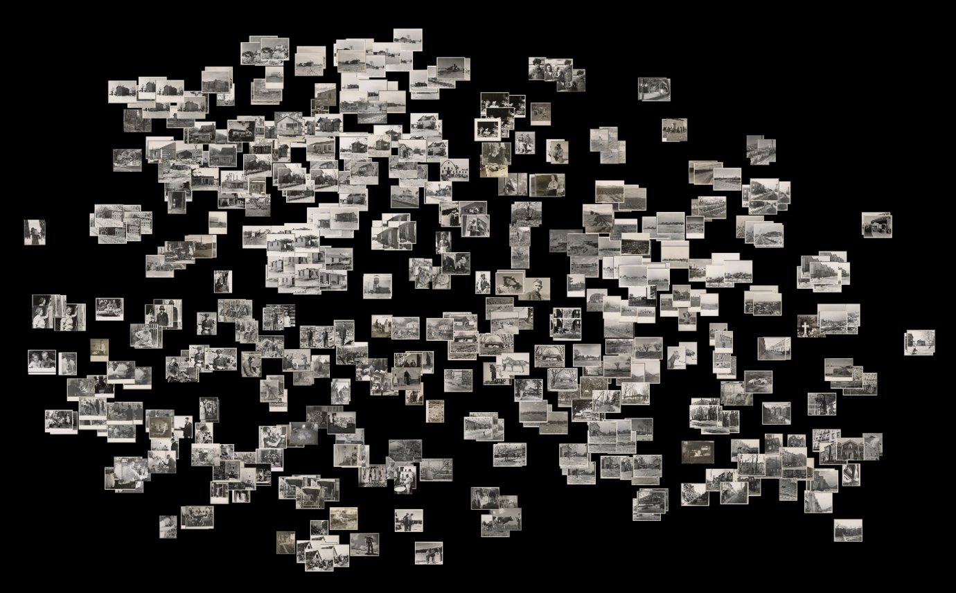
If we load all of the image vectors into a TSNE model then project the data down two two dimensions, we can create a two-dimensional representation of the image collection that preserves similarity between images. Within this representation of the data, each image is positioned near the images to which it’s most similar (click for interactive view):

This plot itself is generated with native HTML5 canvas methods, but D3.js helps provide data fetching, DOM manipulation, and a Voronoi mouseover map. The data for the plot was produced by this tsne clustering script.