An autoencoder is a type of neural network that is comprised of two functions: an encoder that projects data from high to low dimensionality, and a decoder that projects data from low to high dimensionality. To understand how these two functions work, let’s consider the following images:

Since each of these images is 28 pixels by 28 pixels, we can consider each as a 748-dimensional vector (or list of numbers), and can construct an autoencoder in which the encoder projects these 748-dimensional vectors to a two-dimensional vector, just as one might perform dimension reduction using UMAP or TSNE:

While the encoder reduces the dimensionality of input data, the decoder projects samples from low dimensionality back to higher dimensionality. For example, if one constructs a decoder that projects data from 2 dimensions to 748 dimensions, it becomes possible to project arbitrary positions in a two dimensional plane into a 748 pixel image. Click around in the figure below to see how a decoder projects from 2 to 748 dimensions. Note that you can click in areas where there are no samples and the decoder will still generate an image:

An autoencoder is a neural network that combines the encoder and decoder discussed above into a single model that projects input data to a lower-dimensional embedding (the encode step), and then projects that lower-dimensional data back to a high dimensional embedding (the decode step). The goal of the autoencoder is to update its internal weights so that it can project an input vector to a lower dimensionality, then project that low-dimensional vector back to the input vector shape in such a way as to produce an output vector that closely resembles the input vector. One can see a visual diagram of the autoencoder model architecture—and see how the autoencoder’s projections improve with training—by interacting with the figure below:

Having discussed the purpose and basic components of an autoencoder, let’s now discuss how to create autoencoders using the Keras framework in Python.

Building Autoencoders with Keras

To build a custom autoencoder with the Keras framework, we’ll want to start by collecting the data on which the model will be trained. To keep things simple and moderately interesting, we’ll use a collection of images of celebrity faces known as the CelebA dataset. One can download and prepare to analyze 20,000 images from this dataset with the following:

from keras.preprocessing.image import load_img, img_to_array
import requests, zipfile, glob
import numpy as np

# download the images to a directory named "celeba-sample"
url = 'http://bit.ly/celeba-sample'
data = requests.get(url, allow_redirects=True).content
open('celeba-sample.zip', 'wb').write(data)
zipfile.ZipFile('celeba-sample.zip').extractall()

# combine all images in "celeba-sample" into a numpy array
read_img = lambda i: img_to_array(load_img(i, color_mode='grayscale'))
files = glob.glob('celeba-sample/*.jpg')
X = np.array([read_img(i) for i in files]).squeeze() / 255.0 # scale 0:1

Running these lines will create a directory named celeba-sample that contains a collection of 20,000 images with uniform size (218 pixels tall by 178 pixels wide), and will read all of those images into a numpy array X with shape (20000, 218, 178).

With this dataset prepared, we’re now ready to define the autoencoder model. Happily, the Keras framework makes it possible to define an autoencoder including the encode and decode steps discussed above in roughly 25 lines of code:

from keras.models import Model
from keras.layers import Input, Reshape, Dense, Flatten

class Autoencoder:
  def __init__(self, img_shape=(218, 178), latent_dim=2, n_layers=2, n_units=128):
    if not img_shape: raise Exception('Please provide img_shape (height, width) in px')

    # create the encoder
    i = h = Input(img_shape) # the encoder takes as input images
    h = Flatten()(h) # flatten the image into a 1D vector
    for _ in range(n_layers): # add the "hidden" layers
      h = Dense(n_units, activation='relu')(h) # add the units in the ith hidden layer
    o = Dense(latent_dim)(h) # this layer indicates the lower dimensional size
    self.encoder = Model(inputs=[i], outputs=[o])

    # create the decoder
    i = h = Input((latent_dim,)) # the decoder takes as input lower dimensional vectors
    for _ in range(n_layers): # add the "hidden" layers
      h = Dense(n_units, activation='relu')(h) # add the units in the ith hidden layer
    h = Dense(img_shape[0] * img_shape[1])(h) # one unit per pixel in inputs
    o = Reshape(img_shape)(h) # create outputs with the shape of input images
    self.decoder = Model(inputs=[i], outputs=[o])

    # combine the encoder and decoder into a full autoencoder
    i = Input(img_shape) # take as input image vectors
    z = self.encoder(i) # push observations into latent space
    o = self.decoder(z) # project from latent space to feature space
    self.model = Model(inputs=[i], outputs=[o])
    self.model.compile(loss='mse', optimizer='adam')

autoencoder = Autoencoder()

Let’s step through the code above a little. First, we import the building blocks with which we’ll construct the autoencoder from the keras library. Then we define the encoder, decoder, and “stacked” autoencoder, which combines the encoder and decoder into a single model. Each of these models is defined inside a single class that takes as input several named parameters which collectively define the hyperparameters that will be used to define the model. The inline comments above detail how each line contributes to the construction of the encoder, decoder, and stacked autoencoder.

Now that the autoencoder is defined, we can “train” it by passing observations from the numpy array X through the model. Note that we hold out some images from X to use as validation data:

train = X[:-1000]
test = X[-1000:]
autoencoder.model.fit(train, train, validation_data=(test, test), batch_size=64, epochs=1000)

If you run that line, you should see that the model’s aggregate “loss” (or measure of the difference between model inputs and reconstructed outputs) decreases for a period of time and then eventually levels out. Once the loss starts to level out, you can sometimes try to decrease the model’s learning rate and continue training:

import keras.backend as K
K.eval(autoencoder.model.optimizer.lr)
K.set_value(autoencoder.model.optimizer.lr, 0.0001)

Once the model’s loss seems to stop diminishing, we can treat the model as trained and ready for action.

Analyzing the Trained Autoencoder

After training the model, one can analyze the ways the encoder and decoder transform input images. In the first place, we can analyze the way the encoder positions each image in the latent space by plotting the 2D positions of each image in the input dataset:

import matplotlib.pyplot as plt

# transform each input image into the latent space
z = autoencoder.encoder.predict(X)

# plot the latent space
plt.scatter(z[:,0], z[:,1], marker='o', s=0.1, c='#d53a26')
plt.show()

Examining the latent space, you should find that input images are roughly normally distributed around some central point, as in the following example (note however that your visualization may look slightly different due to the random initialization of the autoencoder’s weights):

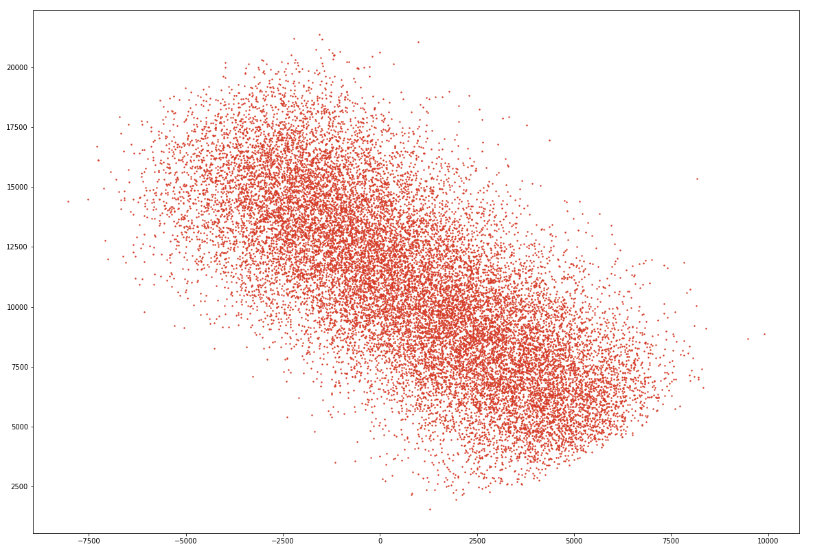
The plot above shows how each image in the input dataset X can be projected into the two-dimensional space created by the middlemost layer of the autoencoder we defined above. What’s arguably more interesting, however, is the decoder’s ability to take positions from that two-dimensional space and project them back up into full-fledged images. Using this ability, one can create new images that are conditioned by, but non-identical to, the input images on which the autoencoder was trained. Let’s visualize some of the outputs from the decoder next.

Sampling from the Latent Space

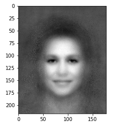
Having trained the autoencoder, we can now pick a random location in the two-dimensional latent space and ask the decoder to transform that two-dimensional value into an image:

# sample from the region 10, 50 in the latent space
import matplotlib.pyplot as plt

y = np.array([[10, 50]])
prediction = autoencoder.decoder.predict(y)
plt.imshow(prediction.squeeze(), cmap='gray')

This will display a face like the following:

Sampling from different regions of the latent space will create rather different faces. To make this sampling process a little more snappy, let’s use Tensorflow.js to create a realtime, interactive decoder.

Exploring Latent Spaces Dynamically

To explore the autoencoder’s latent space in realtime, we can use Tensorflow.js, a stunning open source project built by the Google Brain team. To get started, install the package with pip install tensorflowjs==3.8.0. That command will install a package that includes the resources needed to save a Keras model to disk a format with which the Tensorflow.js clientside library can interact. After that package finishes installing, you should have tensorflowjs_converter on your system path. Using that binary, one can save the decoder defined above to disk by running:

import subprocess, os

model_name = 'celeba' # string used to define filename of saved model
autoencoder.decoder.save(model_name + '-decoder.hdf5', include_optimizer=True)

out_dir = model_name + '-decoder-js'
if not os.path.exists(out_dir): os.makedirs(out_dir)

cmd = 'tensorflowjs_converter '
cmd += '--input_format keras_saved_model '
cmd += model_name + '-decoder.hdf5 '
cmd += out_dir
subprocess.check_output(cmd, shell=True)

This command will create celeba-decoder.hdf5 and celeba-decoder-js, the latter of which is a directory full of files that collectively specify the decoder’s internal parameters. Once those files are saved to disk, one can load the decoder and sample from the position 10, 50 in the latent space (just as we did above) with the following HTML:

<!DOCTYPE html>
<html>
  <head>
    <meta charset='utf-8'>
    <title>Visualizing Autoencoders with Tensorflow.js</title>
  </head>
  <body>
    <script src='https://cdnjs.cloudflare.com/ajax/libs/tensorflow/3.8.0/tf.min.js'></script>
    <script>
    var modelPath = 'celeba-decoder-js/model.json';
    tf.loadLayersModel(modelPath).then(function(model) {
      // convert 10, 50 into a vector
      var y = tf.tensor2d([[10, 50]]);
      // sample from region 10, 50 in latent space
      var prediction = model.predict(y).dataSync();
      // log the prediction to the browser console
      console.log(prediction);
    })
    </script>
  </body>
</html>

To try this snippet out, save the HTML above to a file named index.html and start a local webserver with either python -m http.server 8000 (Python 3) or python -m SimpleHTTPServer 8000 (Python 2). Then open a web browser to the port on which the server you just started is running, namely http://localhost:8000 and inspect the browser console. If you do so, you should see that the lines above log an array of 38,804 values, one value for each pixel in the 178 * 218 pixel image sampled from position 10, 50 in the latent space.

If all this came together, you’re ready to create some interactive models with Tensorflow.js! To do so, we just need to put together a few lines of code that can visualize the array of data returned by the model.predict(y).dataSync() call above. The following will accomplish this goal fairly succintly:

<!DOCTYPE html>
<html>
  <head>
    <meta charset='utf-8'>
    <title>Visualizing Autoencoders with Tensorflow.js</title>
    <style>
      html, body {margin: 0; height: 100%; width: 100%; overflow: hidden;}
    </style>
  </head>
  <body>
    <script src='https://cdnjs.cloudflare.com/ajax/libs/tensorflow/3.8.0/tf.min.js'></script>
    <script src='https://cdnjs.cloudflare.com/ajax/libs/three.js/97/three.min.js'></script>
    <script src='https://duhaime.s3.amazonaws.com/blog/latent-spaces/Controls2D.js'></script>
    <script src='https://duhaime.s3.amazonaws.com/blog/latent-spaces/ThreeWorld.js'></script>
    <script src='https://threejs.org/examples/js/controls/TrackballControls.js'></script>
    <script>
    // get the point geometry
    function getGeometry(colors) {
      var geometry = new THREE.Geometry();
      for (var i=0, y=218; y>0; y--) {
        for (var  x=0; x<178; x++) {
          var color = colors && colors.length ? colors[i++] : Math.random();
          geometry.vertices.push(new THREE.Vector3(x-(182/2), y-(218/2), 0));
          geometry.colors.push(new THREE.Color(color, color, color));
        }
      }
      return geometry;
    }

    // sample from the latent space at obj.x, obj.y
    function sample(obj) {
      obj.x = (obj.x - 0.5) * 500;
      obj.y = (obj.y - 0.5) * 500;
      // convert 10, 50 into a vector
      var y = tf.tensor2d([[obj.x, obj.y]]);
      // sample from region 10, 50 in latent space
      var prediction = window.decoder.predict(y).dataSync();
      // log the prediction to the browser console
      mesh.geometry = getGeometry(prediction);
    }

    // add the mesh to the scene
    var world = new ThreeWorld();
    var materialConfig = { size: 1.25, vertexColors: THREE.VertexColors, };
    var material = new THREE.PointsMaterial(materialConfig);
    var geometry = getGeometry([]);
    var mesh = new THREE.Points(geometry, material);
    world.scene.add(mesh);

    // load the decoder with tensorflow.js and render the scene
    var modelPath = 'celeba-decoder-js/model.json';
    tf.loadLayersModel(modelPath).then(function(model) {
      window.decoder = model;
      sample({x: 0, y: 0})
      world.render();
      new Controls2D({ onDrag: sample });
    })
    </script>
  </body>
</html>

The code above creates an interactive widget like the following:

By interacting with the two-dimensional range slider, users can explore the autoencoder’s latent space, sampling from a continuous range of latent space positions and examining the image the decoder generates for each. That’s all it takes to visualize a latent space with Tensorflow.js!

I want to thank Chase Shimmin, a brilliant physicist and bona-fide machine learning expert, for helping me take a deeper dive into autoencoders. The notes in this post are my humble attempt to circulate some of the insights Chase shared with me among a larger audience.