Working with Professor Matthew Wilkens, my fellow doctoral student Suen Wong, and undergraduates at Notre Dame, I have spent the last few months using the Stanford Named Entity Recognition (NER) classifier to identify locations in a few thousand works of nineteenth-century American literature. Using the NER classifier—an enormously powerful tool that can identify such “named entities” in texts as people, places, and company names—our mission was to find all of the locations within Professor Wilkens’ corpus of nineteenth-century novels. While Stanford’s out-of-the-box classifier could be used for such a purpose, we elected to retrain the tool with nineteenth-century text files in order to improve the classifier’s performance. In case others are curious about the process involved in retraining and testing a trained classifier, I thought it might be worthwhile to provide a quick summation of our method and findings to date.

In order to train the classifier to correctly identify locations in a text, users essentially provide the classifier with a substantial quantity of texts. These texts are annotated in such a way as to teach the classifier to correctly identify locations. More specifically, these “training texts” break a text document into a series of words, each of which users must identify as a location or a non-location. The training files looks a bit like this:

the 0
Greenland   LOC
whale   0
is  0
deposed 0
,   0
-   0
the 0
great   0
sperm   0
whale   0
now 0
reigneth    0
!   0

In this sample, as in all of the training texts, each word (or “token”) is listed on a unique line, followed by a tab and then a “LOC” or a “0” to indicate whether the given token is or is not a location. Users can feed the Stanford parser this data, and the tool can use this information in order to improve its ability to classify locations correctly.

In our training process, we collected hundreds of passages much longer than the sample section above, and we processed those passages in the way described above—with each token on a unique line, followed by a tab and then a “LOC” or a “0”. (Technically, we also identified persons and organizations, but the discussion is made more simple if we presently ignore these other categories.) We then used a quick Python script to sort these hundreds of annotated text chunks into ten directories of equal size, and another script to combine all of the chunks within each directory into a single file.

Once we had ten unique directories, each containing a single amalgamated file, we trained and tested ten classifiers. To train this first classifier, we combined the annotated texts contained in directories 2-10 into a single text file called “directories2-10combined.tsv”. We then created a .prop file we could use to train the first classifier. This .prop file looked very similar to the default .prop template on the FAQ page for the NER classifier:

# location of the training file
trainFile = directoriest2-10combined.tsv
# location where you would like to save (serialize) your
# classifier; adding .gz at the end automatically gzips the file,
# making it smaller, and faster to load
serializeTo = ner-model.ser.gz

# structure of your training file; this tells the classifier that
# the word is in column 0 and the correct answer is in column 1
map = word=0,answer=1

# This specifies the order of the CRF: order 1 means that features
# apply at most to a class pair of previous class and current class
# or current class and next class.
maxLeft=1

# these are the features we'd like to train with
# some are discussed below, the rest can be
# understood by looking at NERFeatureFactory
useClassFeature=true
useWord=true
# word character ngrams will be included up to length 6 as prefixes
# and suffixes only
useNGrams=true
noMidNGrams=true
maxNGramLeng=6
usePrev=true
useNext=true
useDisjunctive=true
useSequences=true
usePrevSequences=true
# the last 4 properties deal with word shape features
useTypeSeqs=true
useTypeSeqs2=true
useTypeySequences=true
wordShape=chris2useLC

We saved this file as propforclassifierone.prop, and then built the classifier by executing the following command within a shell:

java -cp stanford-ner.jar edu.stanford.nlp.ie.crf.CRFClassifier \
-prop propforclassifierone.prop

This command generated an NER model that one can evoke within a shell using a command such as the following:

java -cp stanford-ner.jar edu.stanford.nlp.ie.crf.CRFClassifier \
-loadClassifier ner-model.ser.gz -testFile directoryone.tsv

This command will analyze the file specified by the last flag—namely, “directoryone.tsv”, the only training text that we withheld when training our first classifier. The reason we withheld “directoryone.tsv” was so that we could test our newly-trained classifier on the file. Because we have already hand identified all of the locations in the file, to test the performance of the trained classifier we need only check to see whether and to what extent the trained classifier is able to find those locations. Similarly, after training our second classifier on training texts 1 and 3-10, we can test that classifier’s accuracy by seeing how well it identifies locations in directorytwo.tsv. In general, we can train our classifier on all ten of our training texts save for one, and then test the classifier on that one tsv file. This method is called “ten-fold cross validation,” because it gives us ten opportunities to measure the performance of our training routine and thereby estimate the future success rate of our classifier.

Running the last command listed above generates a text with three columns: the first column contains the tokens in “directoryone.tsv”, the second column contains the “0”s and “LOC”s we used to classify those tokens by hand in our training texts above, and the third column contains the classifier’s guess regarding the status of each token. In other words, if the first word in “directoryone.tsv” is “Montauk”, and we designated this token as a location, but the trained classifier did not, the first row of the output file will look like this:

Montauk LOC 0

By measuring the degree to which the tool’s classifications match our human classifications, we can measure the accuracy of the trained classifier. After training all ten classifiers, we did precisely this, measuring the success rates of each classifier and plotting the resulting figures in R:

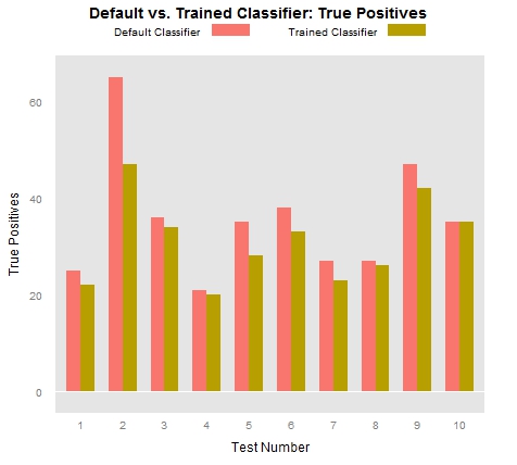
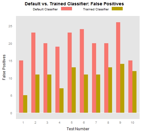
This first plot measures the number of true positive locations that both the out-of-the-box Stanford parser identified in each of our .tsv files as well as the number of true positives our trained classifiers identified in each .tsv file. A true positive location is a token that the classifier has identified as a location (this is what makes it “positive”) that we have also designated as a location (this is what makes it “true”). If the classifier designates a token as a location but we have identified as a non-location, that counts as a “false positive.” The following graph makes it fairly clear that the out-of-the-box classifier tends to produce many more false positives than our trained classifiers:

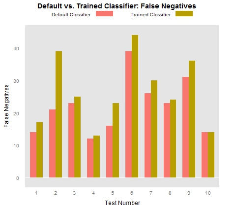
While measuring true positives and false positives is important, it’s also important to measure false negatives, which are tokens that we have identified as locations that the classifier fails to identify as locations. The following graph illustrates the fact that the trained classifier tended to miss many more locations than did the out-of-the-box classifier:

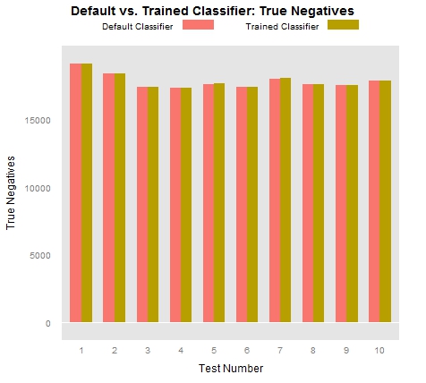
Aside from true positives, false positives, and false negatives, the only other possibility is “true negatives”, which are so numerous as to almost prevent comparison when plotted together:

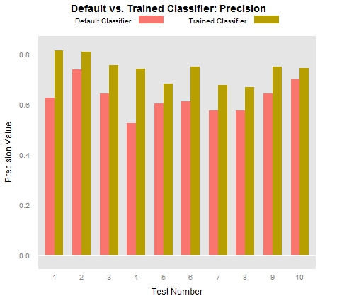
While the plots of true positives, false positives, and false negatives above speak to some of the strengths and weaknesses of the trained classifiers, those who work in statistics and information retrieval like to combine some of these values in order to offer additional insight into their data. One such combination that is commonly employed is called “Precision”, which in our case is a measure of the degree to which those tokens identified as locations by a given classifier are indeed locations. More specifically, precision is calculated by taking the total number of true positives and dividing that number by the combined sum of true positives and false positives (P = TP/TP+FP). Here are the P values of the trained and untrained classifiers:

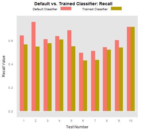
Another common measure used by statisticians is “Recall”, which is calculated by dividing the number of true positives by the sum total of true positives and false negatives (R = TP/TP+FN). In our tests, recall is essentially an indication of the degree to which a given classifier is able to find all of the tokens that we have identified as locations. Clearly the trained classifier did not excel at this task:

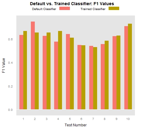
Finally, once we have calculated our precision and recall values, we can combine those values into an “F measure,” which serves as an abstract index of both. There are many ways to calculate F values, depending on whether precision or recall are more important for one’s experiment, but to grant equal weight to both precision and recall, we can use a standard harmonic means equation: F = 2PR/P+R. The F values below may serve as an aggregate index of the success of our classifiers:

So what do these charts tell us? In the first place, they tell us that the trained classifiers tend to operate with much greater precision than the out-of-the-box classifier. To state the point slightly differently, we could say that the trained classifier had far fewer false positives than did the untrained classifier. On the other hand, the trained classifier had far more false negatives than did the untrained classifier. This means that the trained classifier incorrectly identified many locations as non-locations. In sum, if our classifier were a baseball player, it would swing at only some of the many beautiful pitches it saw, but if it decided to swing, it would hit the ball pretty darn well.

It stands to reason that further training will only continue to improve the classifier’s performance. After all, the NER classifier learns from the grammatical structures of the training files it is fed, which allows the classifier to correctly identify locations it has never encountered before. (One can independently prove that this is the case by running a few Python scripts on the data generated by the classifier.) As we continue to feed the classifier additional grammatical constructs that are used in discussions of locations, the classifier should expand its “location vocabulary” and should therefore be more willing to swing at pretty pitches. Once we’ve finished compiling the last two thirds of our training texts, we will be able to retrain the classifiers and see whether this hypothesis holds any water. Here’s looking forward to seeing those results!